1. The Performance Dilemma
You had a long-running (6,000-second) profiling session of a performance-critical function, but pinpointing the precise issue required more insight. Traditional profilers told you where time was spent—but not context. So you created a jsonl trace of 33 GiB containing 384 million data points full with runtime parameters and metrics—only to hit the next roadblock: data ingestion.
Inserting 33 GiB of jsonl into MySQL crawled at under 1,500 inserts/sec—an ordeal that could have taken days. Switching to MemCP via PHP + PDO yielded about 2,000 inserts/sec—still a 53-hour marathon. Even though you used the “sloppy” engine in MemCP to eliminate disk writes, the bottleneck remained the PHP connector.
2. A CSV-Savvy Breakthrough
Converting the giant 33 GiB jsonl to a lean 14 GiB CSV cleared the next hurdle. The PHP conversion completed in just 10 minutes. Then, switching to MemCP’s built-in CSV loader:
(loadCSV (stream "filename.csv"))—3.5 minutes later, it was in-memory, at an extraordinary 1.1 million items/sec load rate.
3. Compression Magic: From 14 GiB to 1.3 GiB
Here’s where MemCP dazzles: those 14 GiB of raw CSV data occupied only 1.3 GiB of RAM—an impressive 10× compression ratio. That’s beyond MySQL-like expectations and reflects MemCP’s intelligent in-memory compression:
- Columnar storage enables compression strategies such as bit-packing, dictionary encoding, and sparse null compression GitHubmemcp.org.
- Typical compression ratios average 1:5, saving 80% memory compared to MySQL/MariaDB memcp.orgGitHub.
Your 10× ratio is even higher, likely thanks to highly repetitive or numerical data patterns—further demonstrating MemCP’s efficiency for analytics.
4. A Shard-Level Peek
After loading the 14 GiB CSV trace into MemCP, the memory footprint was just 1.369 GiB. To understand how that’s possible, let’s look at how MemCP stores data internally. Each shard holds up to ~61k rows and applies column-wise compression. Here are three example shards:
Shard 6253
---
main count: 61440, delta count: 0, deletions: 0
 mode: string-dict[1 entries; 5 bytes], size = 7.833KiB
 cntin: seq[1x int[1]/int[1]], size = 304B
 cntout: seq[1x int[1]/int[1]], size = 304B
 duration: int[15], size = 112.6KiB
 filters: seq[1x int[1]/int[1]], size = 304B
 append: seq[1x int[1]/int[1]], size = 304B
 p: string-dict[1 entries; 17 bytes], size = 7.845KiB
 ---
 ---
 + insertions 40B
 + deletions 48B
 ---
= total 129.6KiB

Shard 6254
---
main count: 61440, delta count: 0, deletions: 0
 mode: string-dict[1 entries; 5 bytes], size = 7.833KiB
 cntin: seq[176x int[20]/int[20]], size = 1.477KiB
 cntout: seq[187x int[6]/int[7]], size = 968B
 duration: int[15], size = 112.6KiB
 filters: seq[161x int[1]/int[2]], size = 680B
 append: seq[176x int[6]/int[7]], size = 928B
 p: string-dict[3 entries; 43 bytes], size = 15.36KiB
 ---
 ---
 + insertions 40B
 + deletions 48B
 ---
= total 140KiB

Shard 6255
---
main count: 5203, delta count: 0, deletions: 0
 filters: int[4], size = 2.617KiB
 append: seq[784x int[6]/int[7]], size = 2.773KiB
 p: string-dict[29 entries; 401 bytes], size = 3.931KiB
 mode: string-dict[3 entries; 19 bytes], size = 1.612KiB
 cntin: seq[811x int[20]/int[14]], size = 4.938KiB
 cntout: seq[800x int[7]/int[11]], size = 3.312KiB
 duration: int[20], size = 12.77KiB
 ---
 ---
 + insertions 40B
 + deletions 48B
 ---
= total 32.15KiB

= total 1.369GiB
Reading the shard stats (with Sequence Compression)
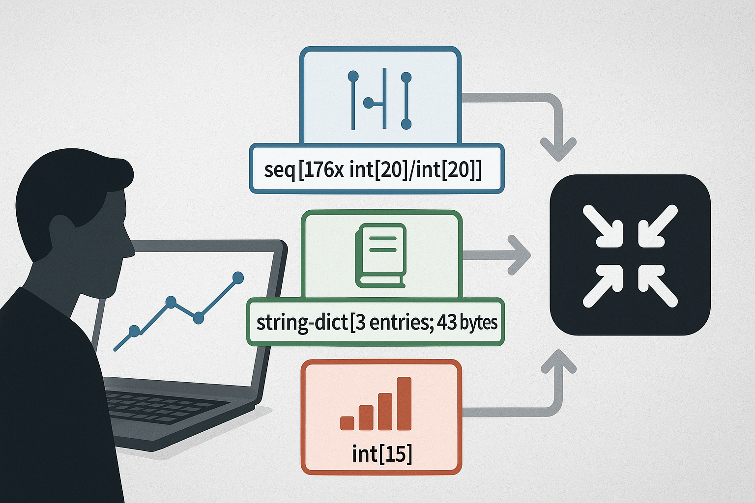
What you’re seeing in the shard dump are MemCP’s columnar storages after compression. Each line shows the container type and how it was compressed:
int[15],int[20]→ bit-packed integer columns where MemCP chooses the minimal bit-width per value based on the column’s min/max. Example:duration: int[15]means each duration uses 15 bits rather than a fixed 32/64-bit slot. This is MemCP’s Integer Compression and it’s why timestamps, IDs, and booleans collapse to a handful of bits per row.string-dict[...]→ dictionary-compressed strings: the column is de-duplicated into a tiny dictionary of distinct values, and the rows store only compact integer codes (which are then bit-packed). That’s howp: string-dict[3 entries; 43 bytes]can encode 61,440 rows with just three distinct strings and ~15 KiB total.seq[... int[a]/int[b]]→ Sequence Compression for integer-like columns that form runs with a constant stride (e.g., auto-increment IDs or counters). Instead of storing every value, MemCP stores sequence descriptors (start, stride, and position metadata for fast random access). The bracket shows how many sequences the column decomposed into and the bit-widths used for the per-sequence integers. Fewer, longer sequences = better compression.
Together, these methods explain the 10× compression ratio you saw: wide trace data with repetitive integers and strings compresses into a fraction of its original footprint.
👉 thanks to this compression, I could run aggregations like SUM(), AVG(), GROUP BY over hundreds of millions of trace entries — interactively, in RAM.
5. Instant Analytics with SQL-Like Power
Now fully loaded, you can run true in-memory analytics—SUM(), AVG(), GROUP BY, filtering, and more—in true OLAP style. Thanks to columnar layout, operations on selected columns avoid unnecessary reads, enabling faster aggregation and memory efficiency.
MemCP handles both OLTP and OLAP workloads seamlessly—no need to copy or transform data between transactional and analytical systems [memcp.org].
Furthermore, compared to MySQL:
- Storage footprint is drastically reduced—80% less for typical workloads [memcp.org].
- You can get up to 10× faster query performance on aggregate operations—perfect for real-time analytics and BI workloads
Here are some example queries:
MySQL [csv]> select count(*) from prefilter where duration is null;
+-------------------+
| (aggregate 1 + 0) |
+-------------------+
|             61439 |
+-------------------+
1 row in set (9,386 sec)

MySQL [csv]> update prefilter set duration = 0 where duration is null;
Query OK, 61439 rows affected (6,138 sec)
MySQL [csv]> select count(*) from prefilter;
+-------------------+
| (aggregate 1 + 0) |
+-------------------+
|    3.84312402e+08 |
+-------------------+
1 row in set (13,658 sec)
MySQL [csv]> select sum(duration) from prefilter;
+--------------------------+
| (aggregate duration + 0) |
+--------------------------+
|       6.816300077497e+12 |
+--------------------------+
1 row in set (16,322 sec)
MySQL [csv]> select p, sum(duration) from prefilter group by p order by sum(duration) DESC;
+---------------------------------------------------+--------------------------+
| p                                                 | (aggregate duration + 0) |
+---------------------------------------------------+--------------------------+
| ExpressionCompileAngular                          |       2.549419217565e+12 |
| Assert                                            |       2.018460559516e+12 |
| ExpressionAngular                                 |         9.7452629555e+11 |
| ExpressionOverwrite                               |        8.28854347601e+11 |
| ExpressionController                              |         2.3639487211e+11 |
| JSONCode                                          |         6.4854399514e+10 |
| ClassMethodCode                                   |         1.3102978222e+10 |
| ClassMethodParameterOrder                         |         1.3045597053e+10 |
| ClassMethodParameter                              |          1.103072277e+10 |
6. Why This Story Matters
My journey showcases how, with MemCP:
- Profiling and tracing becomes feasible at scale when ingestion and storage aren’t bottlenecks.
- Resource savings are real: small RAM, fast ingestion, plus no massive persistent footprint.
- Analytics work becomes interactive: instant queries over dense trace data.
Comments are closed